Daily MJO index time series from 1979
| Index | Description | Obtain timeseries |
|---|---|---|
| CORe VPM The Velocity Potential MJO index. |
Calculated in a similar way as the Wheeler-Hendon RMM, except using 200 hPa Velocity Potential instead of OLR, along with U200 and U850 in a combined EOF (see link to Ventrice et al. 2013 below). This index is computed using the CORe Reanalysis with a climatology based on the years 1991-2020. The correlations with the original VPM index for the overlapping period of 1991-2025 are correlation for PC1 = 0.96858, correlation for PC2 = 0.972385, amplitude correlation = 0.931685. | VPM values |
| ROMI The Real-time OLR MJO Index |
Projection of 9 day running average OLR anomalies onto the daily spatial EOF patterns of 30-96 day eastward filtered OLR. OLR anomalies are calculated by first subtracting the previous 40 day mean OLR. The running average is tapered as the target date is approached. | ROMI values |
| RMII The Realtime Multivariate Index for tropical Intraseasonal oscillations |
Projection of 9 day running average anomalies onto the daily spatial multivariate EOFs of 20-96 day eastward filtered OLR, U850 and U200. Anomalies are calculated by first subtracting the previous 40 day mean. The running average is tapered as the target date is approached. | rMII data currently unavailable. We are working on having this back on the website in the near future. |
| Index | Description | Obtain timeseries |
|---|---|---|
| RMM* The The Realtime Multivariate Madden Julian Index* |
Calculated the same way as the Wheeler-Hendon RMM, but instead of subtracting off the mean of the previous 120 days, a filter based on a linear inverse model (LIM) is applied to remove ENSO variability before projection onto the RMM EOFs. See Marsico et. al. 2025 for further details regarding the LIM filter. The data covers November 1st through April 30th from 1979 to 2021. The file contains all dates with the summer values set to missing. | RMM* values New! |
| OOMI The Original OLR MJO Index |
Projection of 30-96 day eastward only filtered OLR onto the spatial EOF patterns of 30-96 day eastward filtered OLR. This results in a smoother index than OMI due to more restrictive filtering. | OOMI values |
| OMI The OLR MJO Index |
Current OMI uses the NOAA CPC blended OLR. Projection of 20-96 day filtered OLR, including all eastward and westward wave numbers onto the original daily spatial EOF patterns of 30-96 day eastward filtered OLR. This OMI starts in 1991 and is semi-regularly updated to the near-present. | OMI values |
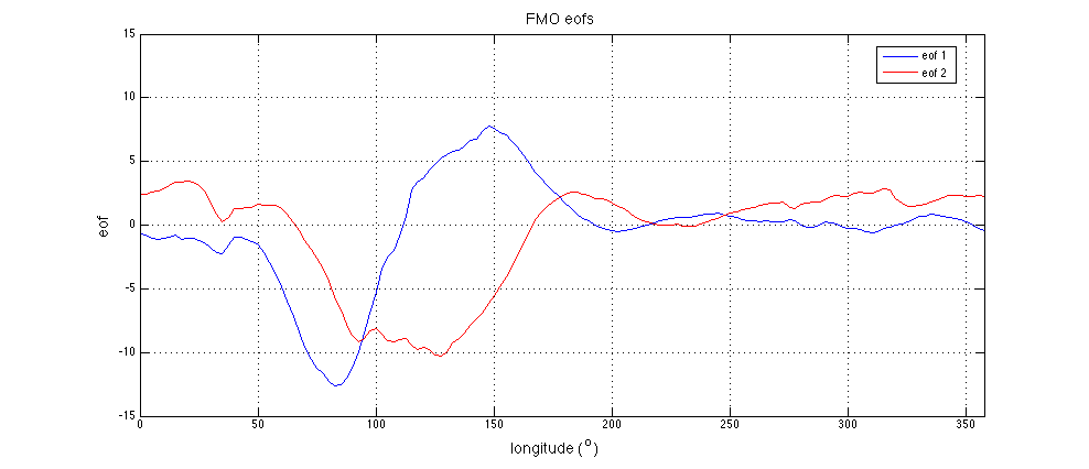
| FMO The Filtered OLR MJO index. |
Univariate EOF of normalized 20-96 day filtered OLR averaged from 15S-15N, by longitude. The same spatial EOF pattern is used for the entire year (see below). | FMO values. |
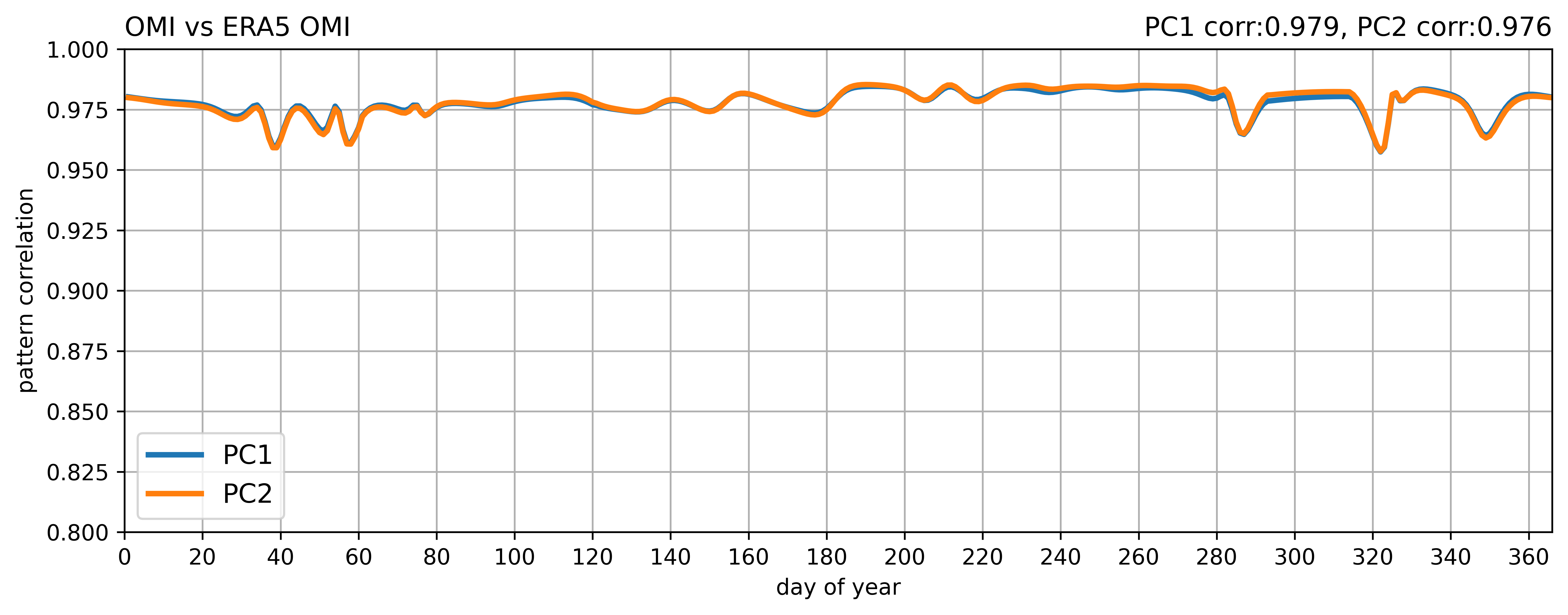
| ERA5 OMI The ERA5 OLR MJO Index |
Projection of 20-96 day filtered ERA5 OLR, including all eastward and westward wave numbers onto the daily spatial EOF patterns of 30-96 day eastward filtered OLR from the ERA5 dataset. EOFs are calculated using data from 1940 to "present". | ERA5 OMI values |
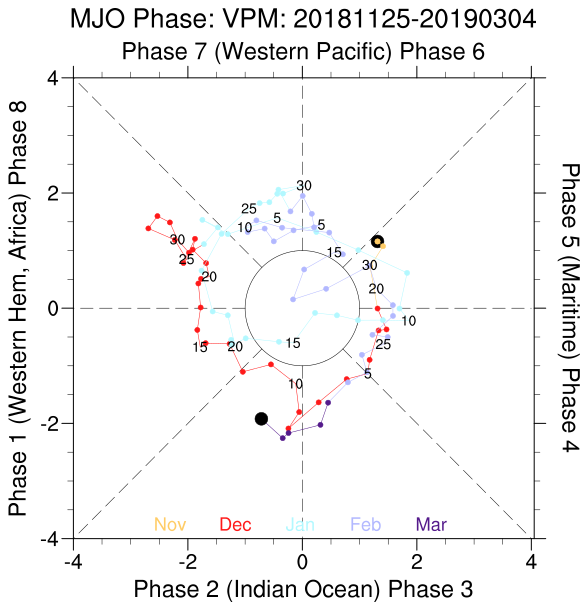
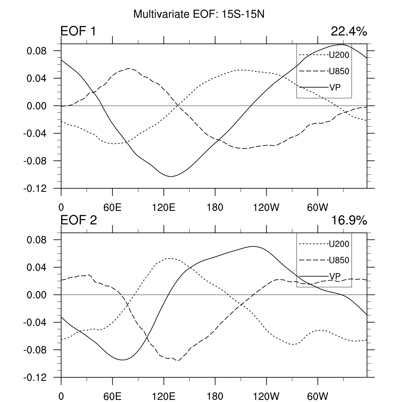
VPM The Velocity Potential MJO index. |
Calculated in the same way as the Wheeler-Hendon RMM, except using 200 hPa Velocity Potential instead of OLR, along with U200 and U850 in a combined EOF (see link to Ventrice et al. 2013 below). This index ends on 2026/03/17 when the NCEP/NCAR Reanalysis Version 1 ended. | VPM values |
| REOMI The Rotated EOFs OLR Madden Julian Index. |
Projection of 20-96 day filtered OLR, including all eastward and westward wave numbers onto the rotated daily spatial EOF patterns of 30-96 day eastward filtered OLR. EOFs are calculated using OLR from 1979-2012. PCs are calculated from 1979-2022. EOFs are rotated to reduce noise and potential degeneracy issues as detailed in Weidman et al., 2022. | REOMI values |
| KRMM The Koopman Real-time MultiVariate Madden Julian Index |
Calculated following the Wheeler-Hendon RMM, but using Koopman spectral analysis to compute eigenfunctions. The leading mode of intraseasonal variability is rotated to maximize correlation with the standard RMM. See link to Lintner et al. 2023 for further discussion of the Koopman spectral analysis and methodological details. | KRMM values |