Meteorological March Madness 2012
Draft - Last Update: 11 December 2012
Disclaimer: This draft is an evolving research assessment and not a final report. The analyses presented have not yet been peer reviewed and do not represent official positions of ESRL, NOAA, or DOC. A more technical and detailed analysis of the heat wave has been submitted to the Bulletin of the American Meteorological Society for peer review. Comments are welcome. For more information, contact Dr. Martin Hoerling (martin.hoerling@noaa.gov)
Anticipation
Credited to various sources including the philosopher David Hume, and discussed by Nassim Taleb in his book "Fooled by Randomness", is the thought that no amount of observations of white swans can allow the inference that all swans are white, but the observation of a single black swan is sufficient to refute that conclusion. The previous sections have shed some light on what appeared to be a "black swan event" (although it is perhaps more than a passing curiosity that at least a "grey swan" occurred in March 1910). Our analysis used standard meteorological data and diagnosis of well-known atmospheric processes. Various hypotheses on this heatwave's plausible causes were tested, some verified, some refuted. Though preliminary and not final in its conclusions, it is demonstrated that much of the heatwave magnitude can be explained from a perspective of elementary physical understanding of the consequences of unusually strong and persistent poleward heat transport by low level southerly winds that extended from the Gulf of Mexico to the Canadian Prairie. Possible relations to La Nina conditions were also explored, and are discussed further below. But all of this begs a critical question; Could the heatwave have been anticipated?, which is the subject of this section.
3. Was this extreme March 2012 U.S. heatwave event anticipated?
Here we explore the evidence for a substantial human influence on the March 2012 heatwave, both on its magnitude and on the probability of such an extreme event occurrence. There is no doubt that there exists an influence of human-produced greenhouse gases on evolving weather and climate conditions, as the IPCC reports have clearly enumerated. Yet, while acknowledging that climate change plays a role in every weather event begs the issue of the direction of that impact and the magnitude of its effect. Unfortunately, when claims are made that a event "would not have happened without human produced greenhouse gases", the incorrect conclusion is all too often drawn by the public and media that an event was caused, in some de novo manner, by human climate change. The pitfall of such framings is apparent from the well-known nature of chaotic weather and climate systems. In that paradigm of a nonlinear system, no event today or tomorrow would have happened owing to the smallest flap of a butterfly's wings. But is there any predictability, and in particular, could the March 2012 heatwave have been anticipated?
|
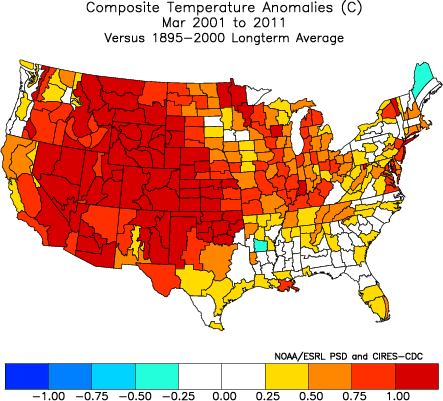
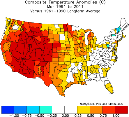
Figure 13: Comparison of the change in monthly averaged March
temperatures for two periods: 1991-2001 compared to the previous 30 years
(top), 2001-2011 compared to the previous century (bottom). [Data source:
NOAA/U.S. Historical Climate Division dataset]
|
Regarding the connection of greenhouse gases and extreme weather, the matter of predictability has often been cast in the context of changed probabilities. As employed in the study of the 2003 European heatwave (Stott et al. 2004) and also the 2010 Russian heatwave (Dole et al. 2011), the question posed is how increased greenhouse gases changed the percent probability of reaching a particular record (or event) threshold. Of course, this is only one aspect of early warning. In the case of the current heatwave, we wish to understand the extent to which GHG forcing offered any of the specificity that characterized the event, namely that it happened in March, that it happen in 2012, that it happen in the Upper Midwest/Ohio Valley region, and that the event had such extreme magnitude. These broader questions, that are at the heart of public interests in early warning, have a rich history in meteorological sciences (e.g., (e.g., Bjerknes 1969; Namias 1982, Miyakoda et al. 1983; Rasmusson and Wallace 1983; Trenberth 1988), but have only recently been applied to the question of climate change impacts of extreme events (e.g., Dole et al. 2011).
While a detailed detection and attribution analysis will be required of the temperature and related climate factors affecting this heatwave's occurrence in March 2012, some initial indications of the plausible magnitude of a greenhouse gas influence on temperatures can be derived from two sources. One is based on data alone, and is presented in Fig. 13. Shown are various estimates of the change in monthly averaged March temperatures, using NOAA's U.S. Historical Climate Division dataset. In one analysis of that data (top panel), the temperature averaged over 1991-2011 is compared to the average over the prior 30-year period. In a second (bottom panel), the average of the first decade of the 21st Century is compared to the 20th Century climatology. Both approaches show a warming U.S. in most areas, with an indication of about a +0.5°C to +1°C increase over the Midwest/Ohio Valley region. The analysis is limited, however, in so far as the single observed record for such a short period of comparison will undoubtedly yield a blend of intrinsic weather noise with a true climate change signal. The true GHG impact on March temperatures, could be greater or less than inferred from Fig. 13.

Figure 14: CMIP5 ensemble average of predicted March 2012 temperatures anomalies (relative to 1980-2010 climatology).
|
A further analysis is thus required, and this necessarily involves the global climate models subjected to the change in GHGs, aerosols and other external forcing. Here we use the newly available CMIP-5 model data that will be part of the modeling input used in the upcoming IPCC Fifth Assessment. Shown in Fig. 14 is the projection of March 2012 temperatures as derived from the ensemble average of 20 different global models. These are projections for 2012 in the sense that they are driven only by a business-as-usual scenario for the GHG emissions. These model experiments are to be distinguished from predictions that would further constrain a model with the actual initial observed state of the climate system in 2012. Predictions based on operational forecast models will be presented and discussed further below.
The 20-member ensemble mean of the projections provides the best current estimate of the modeled GHG impact, and that signal shows a U.S. continent wide warming on the order of +0.5°C to +1.0°C (calculated relative to the models' 1981-2010 climatology). This magnitude of projected warming bears considerable similarity to the magnitudes of trends in surface temperature derived from the two observational approaches, though some regional differences in patterns are apparent. The key point to note is that the CMIP-5 signal of a GHG influence on March 2012 temperatures is roughly in the range of +0.5°C to +1°C warming. However, the signal of climate change in March temperatures over the Midwest/Ohio Valley region is likely not yet detectable because the standard variability of daily March surface temperatures over the Midwest/Ohio Valley region (see Fig. 7, as inferred from 850mb data) is at least 6°C, and that the standard variability of monthly averaged March temperatures (see Fig. 6) is at least 2°C, both appreciably larger than the estimate signal.
What is also important to recognize is that the GHG warming signal for March 2012 offers few of the attributes that are required of a meaningful early warning. First, it fails to anticipate the event happening in 2012, since a similar warming signal existed in 2010 and 2011 (and is again anticipated in 2013), Second, it fails to anticipate the particular monthly occurrence in March, since a similar warming signal exists throughout the annual cycle. Third, it fails to anticipate the specific location of the 2012 heatwave over the Upper Midwest/Ohio Valley region since the magnitude of the GHG signal is not materially different for the western U.S., central U.S., and eastern U.S., or for that matter for Alaska, and Asia which, during this period, experienced severe cold. And, the GHG warming signal fails to explain the extreme magnitude of the heatwave event, which achieved daily departures of +20°C, or about 20-fold greater than the estimated background warming signal. Our physically based analysis explored the possibility for strong nonlinear amplifying feedbacks or highly nonlinear dynamical sensitivity to GHG forcing, and these models which represent such process in their integration of the coupled climate system, are consistent with that empirical assessment that such processes were unlikely of primary significance over the U.S. during March 2012.
The weak overall contribution of GHG warming to the magnitude of the March 2012 heatwave notwithstanding, a signal of about +1°C warming appreciably increased the odds of a record March heatwave occurring. Such a signal corresponds approximately to a 0.5 standardized shift of the probability distribution toward warmer conditions. There are, however, statistical challenges in estimating how such a shift in distributions would alter extreme event odds, especially of the intensity observed in March 2012 whose magnitude was likely on the order of 4 - 6 standard deviations. The limited length of the available data records makes it difficult to discern the nature of the frequency distribution from which our extreme March 2012 heatwave event was drawn. Compounding the difficulties is the extreme sensitivity in estimating changes in probabilities of threshold exceedences to the assumed background distribution. The typical assumptions of a normally distributed (Gaussian) temperature distribution does not hold for daily values in particular. Nor do they generally hold for monthly averaged data when considering the extreme tails of distributions. This issue of estimating reliable statistics of extreme, rare events continues to be a matter of active research. The assumption of Gaussianity is more defensible, however, if considering a threshold of more moderate magnitude. Here we consider the changing odds of exceeding a threshold for a 2 standard deviation departure (~4°C) March temperature condition. This is roughly akin to a 1 in 40 year event magnitude. For a 0.5 standardized anomaly of GHG warming (+1�C), the exceedence probability increases roughly by 50%, and somewhat less than a doubling in the probability.
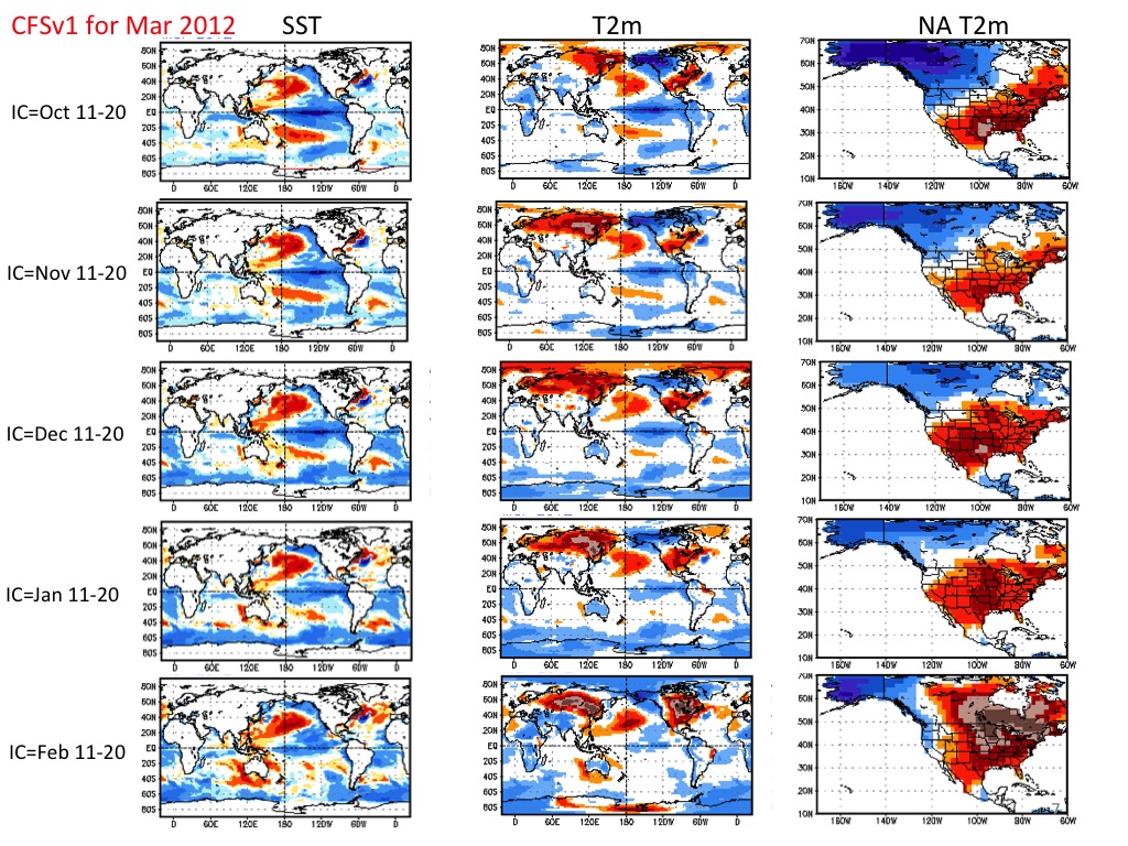
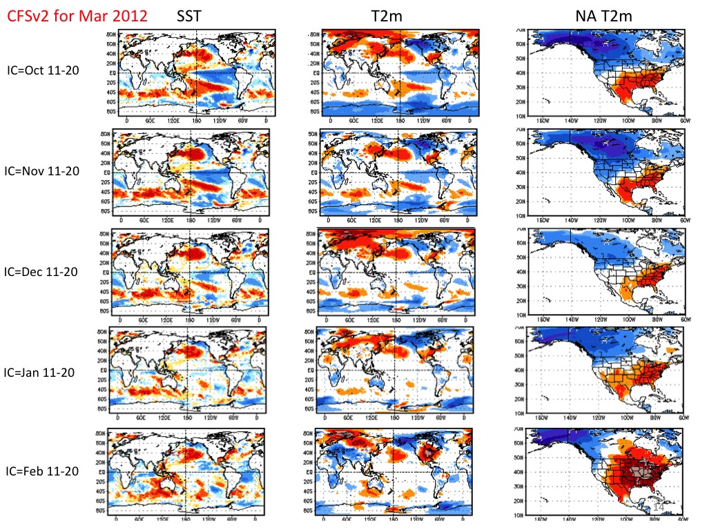
Was there other information, aside from a background GHG warming, that may have caused one to anticipate the March 2012 heatwave? Many of the shortcomings of relying upon GHG forced projections alone as a basis for anticipating the March 2012 heatwave are overcome when relying upon the initialized predictions generated by operational forecast models for this case. This distinction between the climate projections and the climate predictions for March 2012 also strengthens various conclusions based on physical process understanding of the principal causes for the March 2012 heatwave. Here we present a sequence of monthly initialized NOAA/NCEP climate predictions for the verifying month of March 2012. The initializations are done 4 times daily of the ocean, atmosphere, land surface conditions. Shown in Fig. 15a and Fig. 15b are successive initializations from October 2011 to February 2012 for two parallel operational prediction systems run in NOAA. The key feature of the evolving predictions is a sudden and abrupt emergence of a very warm March prediction for the Upper Midwest/Ohio Valley region in the February initialized forecasts. These are substantial changes statistically because each plot represents a 40-run average. Prior forecasts had anticipated warm conditions mostly along the southern tier of the U.S., consistent with the impact of ongoing cold tropical Pacific SSTs associated with a La Nina event.
|
|
| a) CFS v1 | b) CFS v2 |
|---|---|
|
Figure 15: Predictions for March 2012 from a) CFSv1 and b)
CFSv2 using initialized conditions (IC) during the prior 5 months.
| |
The sudden change in location and in magnitude of warming, as anticipated by February initialized forecasts ,reveals the role of an emerging state of internal atmospheric variability. This change is irreconcilable with changes in GHG forcing whose time scale is far too long, and whose influence would have been very similar in the prior initialized forecasts. What is also striking is that the 40-run ensemble mean magnitudes were on the order of +4°C for the monthly March average, which equates to about 2 standardized departures in the forecasts. One can repeat the analysis of how such a magnitude signal (in this case, the signal of the climate prediction rather than the projection) altered the odds for a 2 standardized (i.e. ~4°C) March heatwave. Such a major shift of the distribution in the CFS implies a roughly 10-fold increase in the probability of such a heatwave occurring.
In sum, the initialized forecasts possess many of the essential attributes of what crime scene investigators would look for in pinning a crime (the heatwave, in this case) to an individual (a physical cause, in this case). The forecast models give probable cause, namely that a particular atmospheric initial condition - emergent sometime in early February - led to a high probability outcome in the form of a large magnitude March heatwave. The sequence of forecasts allows one to largely reject other probable and immeditate causes for such a large magnitude event. For example, the GHG conditions that were known to be operative in prior months, had failed to predict or project an outcome of the magnitiude that was eventually observed. The forecasts further identify this particular culprit because those evolving internal atmospheric initial conditions yielded the precise location of the heatwave, at precisely the particular time of its occurrence, and with a high confidence of exceeding prior record heatwave magnitudes.
Epilogue
A black swan most probably was observed in March 2012 (lest we forget 1910). Gifted thereby to a wonderful late winter of unprecedented balmy weather, we also now know that all swans are not white. The event reminds us that there is no reason to believe that the hottest, "meteorological maddest" March observed in a mere century of observations is the hottest possible. But this isn't to push all the blame upon randomness. Our current estimate of the impact of GHG forcing is that it likely contributed on the order of 5% to 10% of the magnitude of the heat wave during 12-23 March. And the probability of heatwaves is growing as GHG-induced warming continues to progress. But there is always the randomness.
Acknowledgements
Thanks to Randy Dole, Jon Eischeid, Stephanie Herring, Arun Kumar, Don Murray, Judith Perlwitz, Robin Webb and Klaus Wolter for their comments, analysis, plots, and data sets.