Extended Multivariate ENSO Index (MEI.ext)
| Click to enlarge |
 |
Outline for MEI.ext webpage (first edition on May 10th, 2011)
1. A short description of the extended Multivariate ENSO Index (MEI.ext);
2. Historic La Niña events before 1950;
3. Historic El Niño events before 1950;
4. MEI.ext loading maps;
5. Publications and MEI.ext data access.
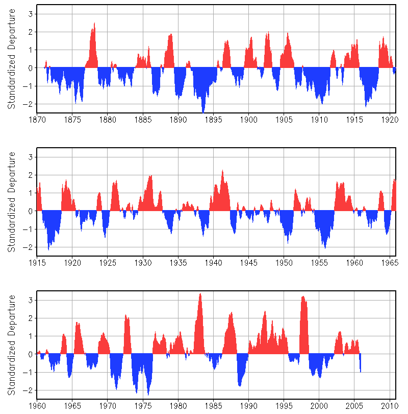
El Niño/Southern Oscillation (ENSO) is the most important coupled ocean-atmosphere phenomenon to cause global climate variability on interannual time scales. Here we attempt to create a reliable ENSO index for much of the historical record by basing the extended Multivariate ENSO Index (MEI.ext) on the two main observed variables over the tropical Pacific that have been reconstructed by the Hadley Centre back to 1871. These two variables are: sea-level pressure (P; details in Allan and Ansell, 2006), and sea surface temperature (S; details in Rayner et al., 2006). Similar to the original MEI, the extended MEI.ext is computed separately for each of twelve sliding bi-monthly seasons (Dec/Jan, Jan/Feb,..., Nov/Dec). Since the original Hadley Centre data are already pre-filtered, the MEI.ext is calculated directly from the gridded fields as the first unrotated Principal Component (PC) of both P and S. This is accomplished by normalizing the total variance of each field first, and then performing the extraction of the first PC on the co-variance matrix of the combined fields (Wolter and Timlin, 2011). The figure above is taken from this paper and shows the bimonthly values of the MEI.ext, standardized with respect to each season, and to the 1871-2005 reference period. Caution should be exercised when interpreting the MEI.ext on a month-to-month basis, since it was developed mainly for research purposes, similar to the original MEI. Negative values of the MEI.ext represent the cold ENSO phase, a.k.a. La Niña, while positive MEI.ext values represent the warm ENSO phase (El Niño).
This website is not intended to replace the original MEI which will continue to be updated monthly into the foreseeable future, while the MEI.ext will remain 'frozen' for now, except for layout changes. In fact, I welcome feedback at (Klaus.Wolter@noaa.gov).
Click on the "Publications and MEI.ext data" button below to gain access to the MEI.ext time series.
Historic La Niña events before 1950
| Click to enlarge |
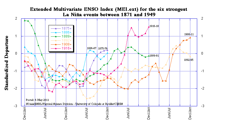 |
How do the six strongest pre-1950 La Niña events compare against each other? This figure includes only events with at least three bimonthly rankings in the top 10% from 1871-1949 (rankings for the full period 1871-2005 are listed here). La Niña events lasted up to and over three years, similar to the mid-1950s and mid-70s events. It is striking that there were no significant La Niña events between 1918 and 1949, a period that is well known for diminished ENSO activities (noted for instance in Trenberth and Shea, 1987). The two longest events with a total of 22 bimonthly seasons each in the top-10%ile stretched from 1892-95 and 1908-11.
Click on the "Publications and MEI.ext data" button below to gain access to the MEI.ext time series.
Historic El Niño events before 1950
| Click to enlarge |
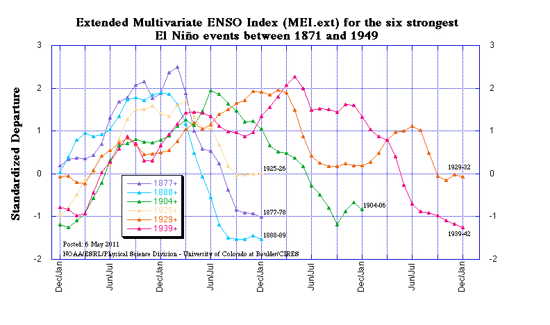 |
How do the six strongest pre-1950 El Niño events compare against each other? This figure includes only events with at least EIGHT bimonthly rankings in the top 10% from 1871-1949 (rankings are listed here). This includes the strongest known event of the 19th century in 1877-78. The high count of at least eight rankings in the top 10% was required to limit the total number of events to six. Shorter strong events with at least three bimonthly rankings in the top 10% clustered around the turn of the century (1896-97, 1899-1900, and 1902-03), as well as during the First World War (1914-15 and 1918-19). While most El Niño events run shorter than comparable La Niña events, it is striking to find the two longest El Niño events (1929-32 and 1939-42) in the middle of the aforementioned low ENSO activity stretch from 1918-1949 (Trenberth and Shea, 1987).
Click on the "Publications and MEI.ext data" button below to gain access to the MEI.ext time series.
MEI loading maps
| Click to enlarge |
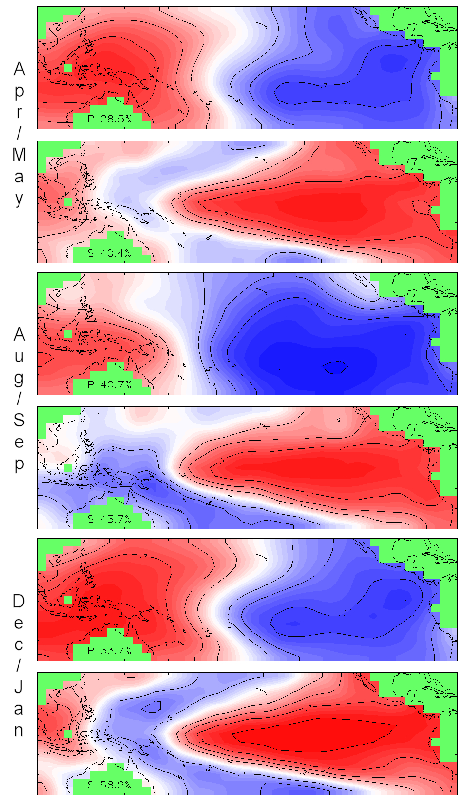 |
While other ENSO indices remain fixed in their spatial definition, the MEI (and MEI.ext) allows for geographic variations in its seasonal features. The above figure is reproduced from Wolter and Timlin, 2011, and documents the loading fields of MEI.ext for 3 out of 12 seasons (April-May, August-September, and December-January) during the full period of record (1871-2005). 'Loadings' represent the linear correlation coefficients between time series of gridded local anomalies and the MEI.ext. Land areas and Atlantic data were masked out in green. Similar to the MEI, each variable is denoted by a single letter, and shows the explained variance for the same field in the 'Australian corner'.
In all seasons, the sea level pressure (P) loadings reveal the familiar dipole pattern of the Southern Oscillation (SO): high pressure anomalies in the west and low pressure anomalies in the east correspond to positive MEI values, or El Niño-likei conditions. During April-May (top panel), the latitudinal position of the highest loadings (or 'centers of gravity', see Wolter and Timlin, 1993) is furthest north (near the Equator) for both poles of the SO when they are also furthest away from Tahiti and Darwin, respectively. This is the season with the lowest explained variance in P. Four months later (middle panel), the highest loadings have shifted back south towards the classic dipole position of the SO during August-September when the total explained variance in P reaches its annual peak. In boreal winter (bottom panel), the pressure dipole shows its highest east-west symmetry. Compared to the original MEI, the explained variance of these bimonthly fields is higher in all seasons, most likely due to the pre-filtered nature of the Hadley Centre data (Allan and Ansell, 2006). This is probably also responsible for the smaller geographic variations in the positions of the centers of gravity of the SO in the MEI.ext compared to the MEI.
The sea surface temperature field (S) exhibits the typical ENSO signature of a near-equatorial wedge of positive loadings stretching from the Central and South American coasts to slightly west of the dateline, or warm anomalies during an El Niño event. To the north- and southwest, a horseshoe-like feature of negative loadings indicates the well known tendency for opposite SST anomalies to occur east of Australia and east of the Philippines (Rasmusson and Carpenter, 1982), stretching into the subtropics of both hemispheres. These negative loadings peak northeast of Australia during austral spring (middle panel). Positive loadings are highest during the boreal winter season (bottom panel), and focus on the Equator between 180 and 100W throughout the year, always encompassing the Niño 3.4 region (120-170W, 5N-5S). A dropoff in loading strength from about Galapagos eastward to South America is apparent in boreal winter and spring (bottom and top panels, respectively). This is consistent with the lack of strong correspondence between near-coastal El Niño events in the traditional sense (Quinn and Neal, 1992) and the basin-wide phenomenon that we are trying to document here. As in P, the explained variance of all seasonal S fields in MEI.ext is higher than in the original MEI, but not by much, and its peak loadings do not move around as much as in the MEI.
The MEI.ext explains between 33% and 47% variance in May-June and October-November, respectively (not shown here). This seasonality is very similar to the MEI which varies between 18% in May-June and 33% in November-December, but includes four other variables (zonal and meridional surface wind, air temperature, and total cloudiness) which reduce the overall explained variance in the original MEI.
MEI.ext data access and publications
You can find the numerical values of the MEI.ext timeseries under this link, and historic ranks under this related link. If you are just interested in the period since 1950, I would recommend visiting the MEI website to get a monthly updated perspective on recent ENSO conditions compared to the ENSO record since 1950.
If you have trouble getting the data, please contact me under (Klaus.Wolter@noaa.gov)
You are welcome to use any of the figures or data from the MEI websites, but proper acknowledgment would be appreciated. Please refer to the (Wolter and Timlin, 2011) paper below.
Publications
- Allan, R.J., and T. Ansell, 2006: A new globally complete monthly historical gridded mean sea level pressure dataset (HadSLP2): 1850-2004. J. Climate, 19, 5816-5842.
- Quinn, W.H., and V.T. Neal, 1992: The historical record of El Niño events. In Climate since A.D. 1500, Bradley, R.S., and P.D. Jones (eds). Routledge: London; 623-648.
- Rayner, N.A., Brohan, P., Parker, D.E., Folland, C.K., Kennedy, J.J., Vanicek, M., Ansell, T.J., and S.F.B. Tett, 2006: Improved analyses of changes and uncertainties in sea surface temperature measured in situ since the mid-nineteenth century: The HadSST2 dataset. J. Climate, 19, 446-469.
- Rasmusson, E.G., and T.H. Carpenter, 1982: Variations in tropical sea surface temperature and surface wind fields associated with the Southern Oscillation/El Niño. Mon. Wea. Rev., 110, 354-384. Available from the AMS.
- Trenberth, K.E., and D.J. Shea, 1987: On the evolution of the Southern Oscillation. Mon. Wea. Rev., 115, 3078-3096.
- Wolter, K., and M.S. Timlin, 1993: Monitoring ENSO in COADS with a seasonally adjusted principal component index. Proc. of the 17th Climate Diagnostics Workshop, Norman, OK, NOAA/NMC/CAC, NSSL, Oklahoma Clim. Survey, CIMMS and the School of Meteor., Univ. of Oklahoma, 52-57. Download PDF.
- Wolter, K., and M. S. Timlin, 2011: El Niño/Southern Oscillation behaviour since 1871 as diagnosed in an extended multivariate ENSO index (MEI.ext). Intl. J. Climatology, 31, 14pp., in press. Available from Wiley Online Library.