PSL generates experimental forecasts on time-scales of weeks to seasons as part of its research mission.
The forecasts and associated information such as verifications are available on the following webpages. It
is planned that these forecasts will eventually be transitioned to operational mode.
| Description | Sample Product |
|---|
-
Arctic sea-ice experimental forecast
-
Experimental, sea ice forecasts produced from a fully coupled ~9km ice(CICE5)-ocean(POP2)-land(CLM4.5)-atmosphere(WRF3.5) model called RASM-ESRL. The model is initialized with the NOAA Global Forecast System (GFS) analyses, CRYOSAT2 sea ice thickness, and Advanced Microwave Scanning Radiometer 2 (AMSR2) sea ice concentrations. The model is forced at the lateral boundaries by 3-hourly GFS forecasts of winds, temperature, and water vapor.
|
|
-
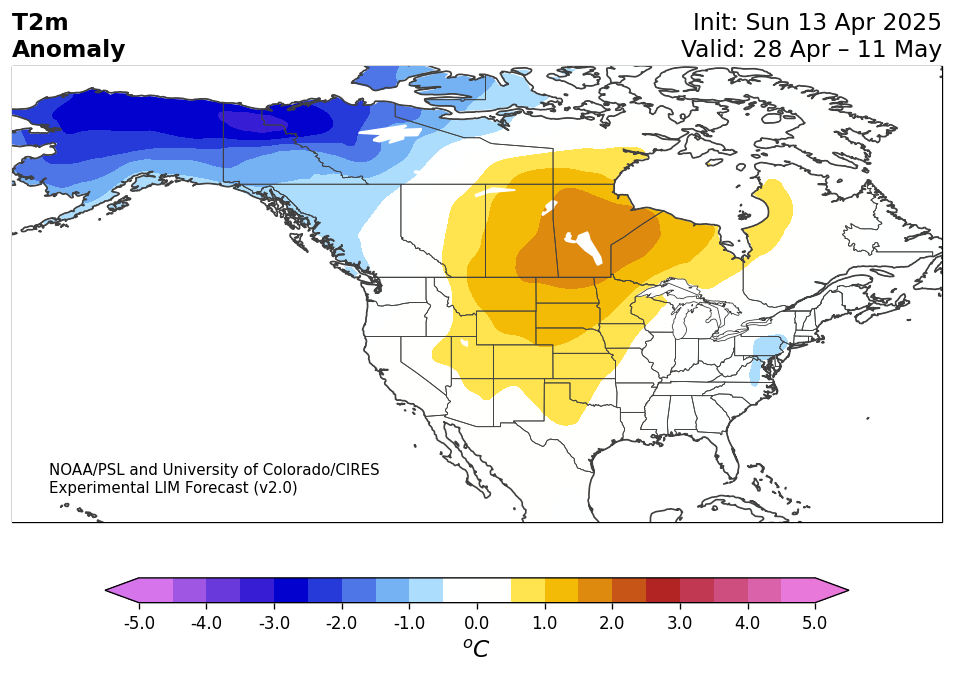
Experimental Probabilistic LIM Subseasonal Linear Inverse Model (LIM) forecasts (weeks 1-6).
-
A empirical dynamical technique, linear inverse modeling is used to create N. American subseasonal forecasts. The model is LIM is trained on Japanese Reanalysis Three Quarters of a Century Reanalysis (JRA-3Q) between 1958-2016 and a number of variables are available including 2m temperature, soil moisture, SLP, and more.
|
|
-
C3S Monthly to Seasonal Forecasts
-
PSL provides monthly and three-monthly (seasonal) forecasts for sea surface temperature, 200-hPa geopotential heights, 2-m temperature, and precipitation. These forecasts are derived from the hindcasts (retrospective forecasts) and current forecasts of five dynamical models. Users can customize their view by selecting a region, initialization date, lag, forecast period, and statistics type.
|

|
-
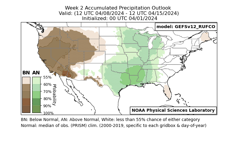
Experimental Subseasonal Precipitation Accumulation Outlooks
-
Experimental subseasonal outlooks (week 1, week 2, and combined weeks 3-4) are provided to demonstrate near real-time performance of conventional and deep-learning-based methods to calibrate raw precipitation accumulation forecasts from NOAA’s Global Ensemble Forecast System version 12. Forecasts are presented as probabilities. Three methods are shown: raw GEFS output, CSGD post-processed guidance, and "RUFCO" neural-network post-processed guidance. Also included are hindcast skill scores and near real-time verification metrics.
|
|
-
GEFSv12 Quantile Mapping
-
The precipitation forecasts apply a quantile-mapping (QM) and dressing routine to bias correct raw quantitative precipitation forecasts (QPF) from NOAA’s Global Ensemble Forecast System version 12 (GEFSv12. The method was designed to improve precipitation in NOAA’s National Blend of Models that incorporates the GEFSv12 30-member ensemble into its forecast guidance. US precipitation forecast maps and netCDF output files are available. Forecasts are made up to 240h from the initialization time. Means and probabilities are forecasted.
|

|
-
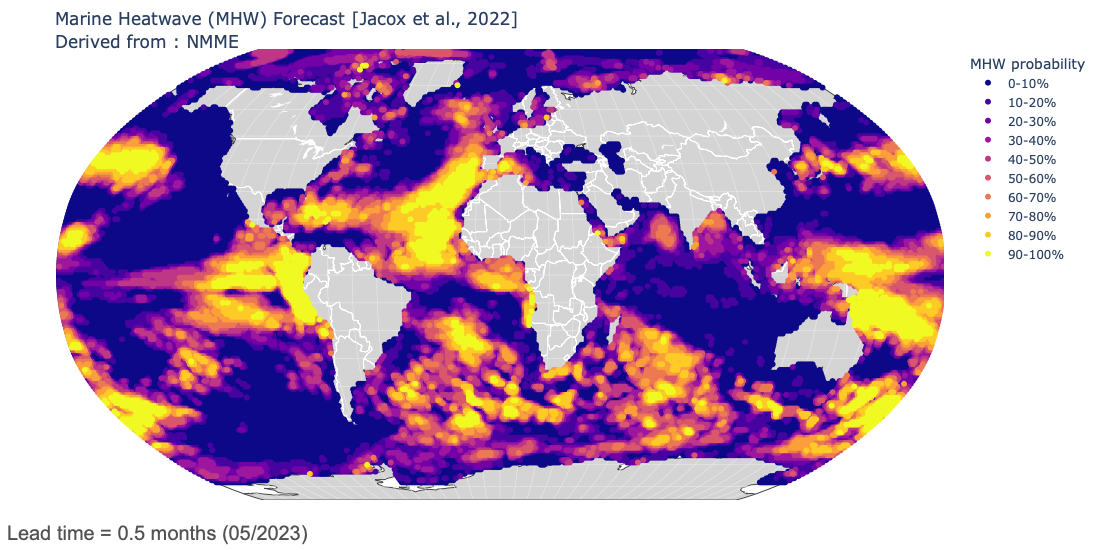
Marine Heatwave Forecasts
- Experimental marine heatwave forecasts produced using sea surface temperature output from six global climate forecast systems contributing to the North American Multi-Model Ensemble (NMME). Forecasts provide global outlooks of marine heatwave probability for the next 12 months. Forecasts are updated monthly, and historical forecasts are available starting in 1991.
|
|
-
Model-Analogs (MA) and Linear Inverse Model (LIM) forecasts for Months 1-24
-
Experimental forecasts of numerous tropical fields, including precipitation, outgoing longwave radiation (OLR), sea surface temperature (SST), and sea surface height (SSH).
Current Month 6 MA precipitation forecast and Niño3.4 Months 1-24 forecast from all models.
|

|
-
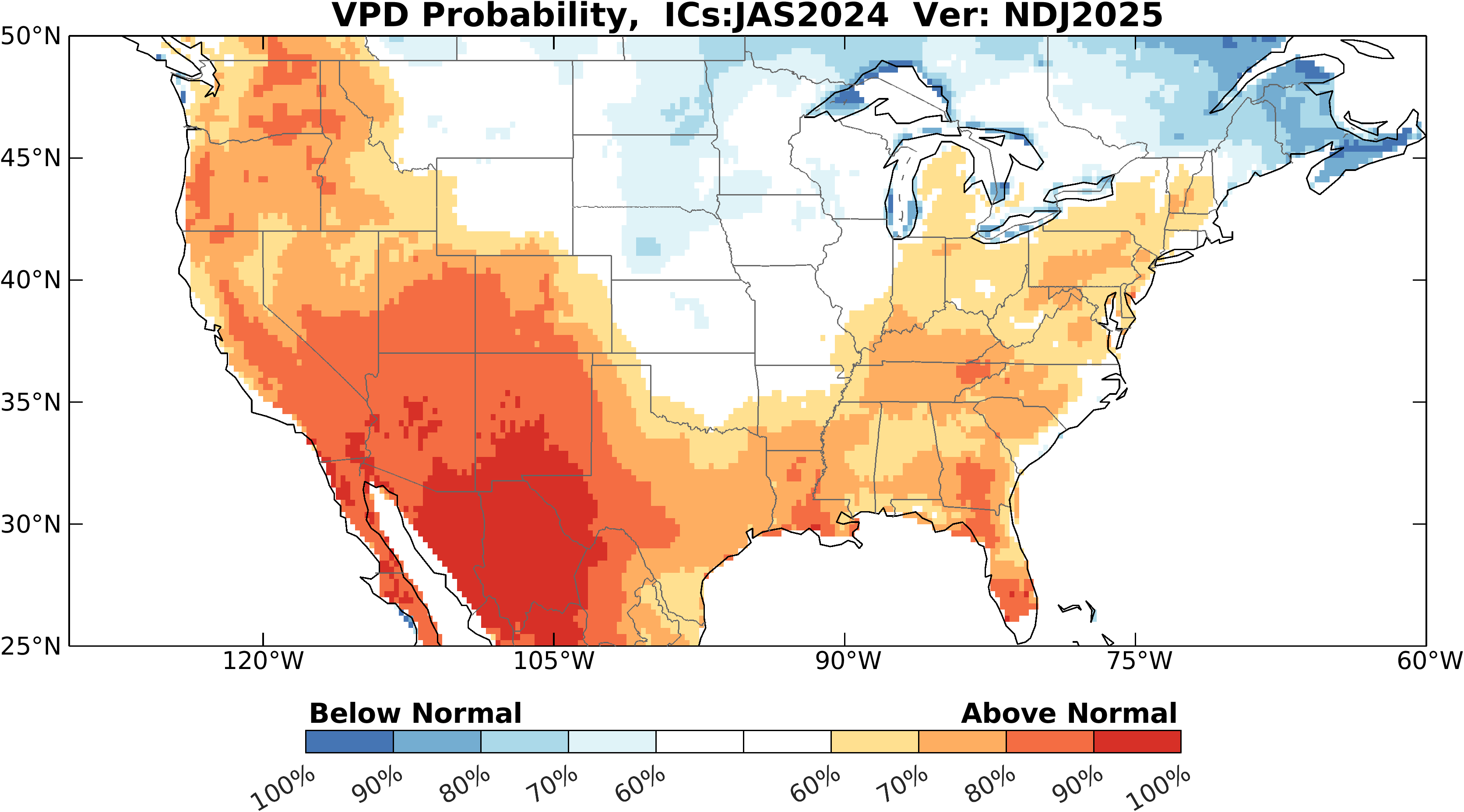
Seasonal Vapor Pressure Deficit (VPD) Guidance
- The Physical Sciences Lab provides experimental vapor pressure deficit (VPD) guidance to provide information that can be used in fire weather risk scenario development. These forecasts are based on a machine learning approach using a linear inverse model. The LIM relies on observed relationships between model variables to infer predictable Earth system processes and generate probabilistic forecasts. Variables used are from the ERA5 reanalysis. Forecasts are provided for a set of 3 months seasons and consist of maps of the probability of VPD being above or below normal relative to the 1991-2020 average. There is a also a version of the forecast that is detrended.
|
|