Directions for WRIT Seasonal Correlation Mapping
Topics:
Variable: Datasets | Variables | Year Range | Season | Lead/Lag |
Statistic
Plotting Options: Plot Type | Map Region | Map Projection | Color/Contours| Reverse Colorbar| Fill Type | Contour interval
Custom Timeseries File
Information: Page Creation | Feedback | Caveats
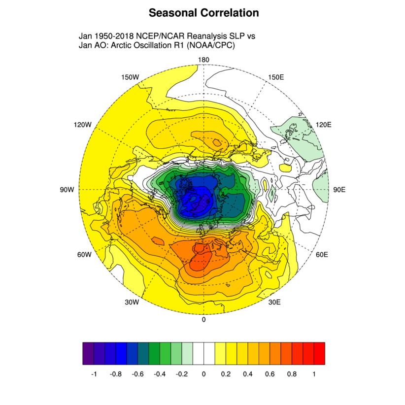
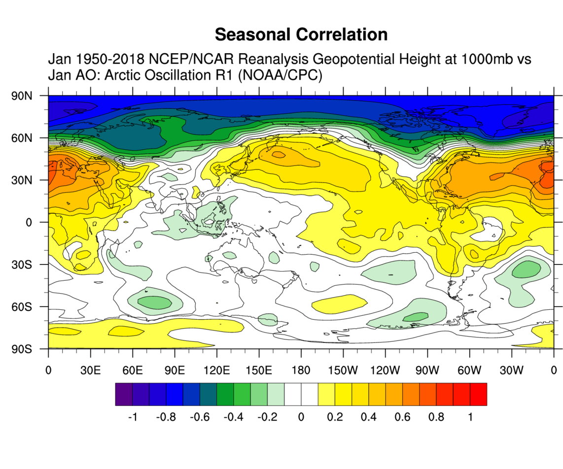
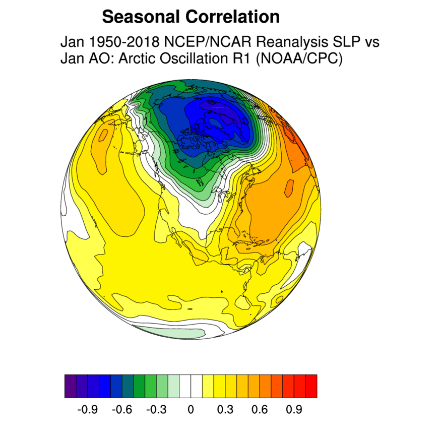
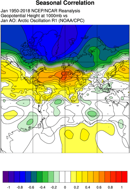
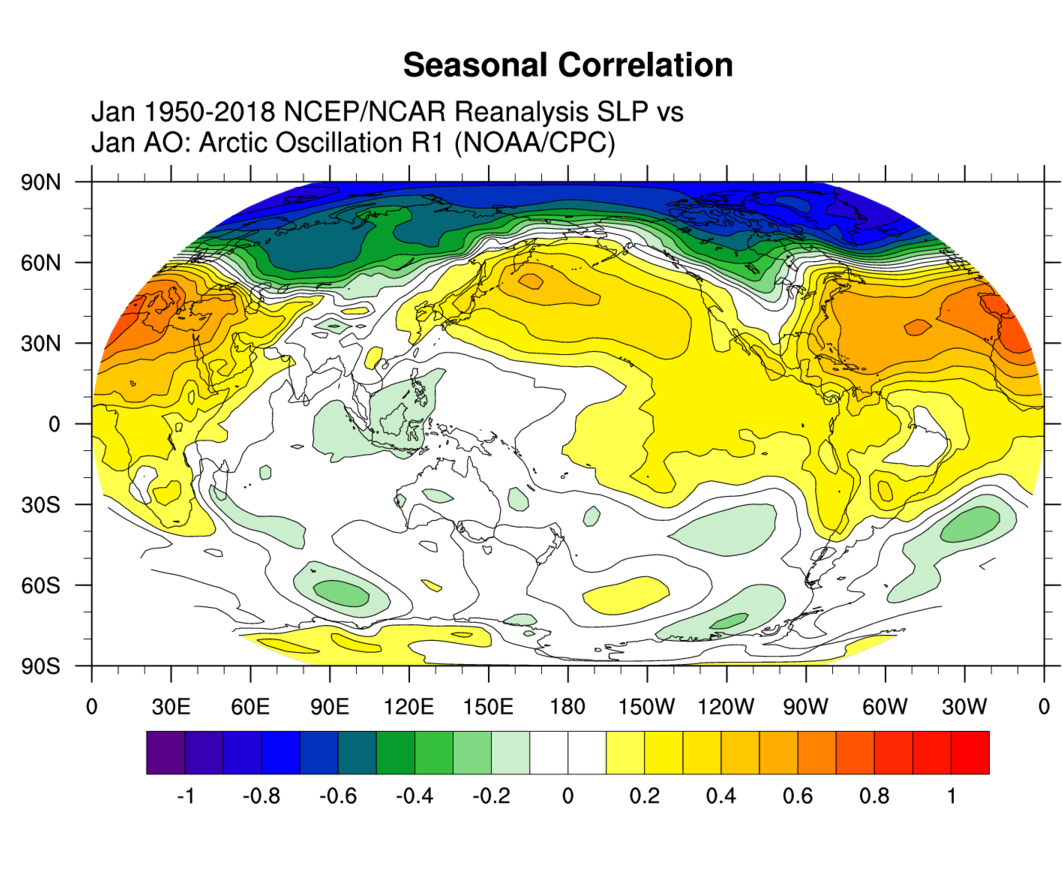
Page will plot correlation maps at a selected pressure level variables or single level variables. Select desired options and hit "create plot". Most options have a default setting so a selection is not required. If you have problems, please email with ALL the options you chose. A plot, the data used to create the final plot (in netCDF), a post script image and information on the dataset will be returned.
| Variable Selection |
|---|
DatasetVarious global reanalyses and observational datasets are provided. For the MERRA and MERRA-2, we are using the lower resolution data (1.5x1.5). MERRA/MERRA-2 are not defined for values below the surface (details). All other reanalyses datasets we provide have values for the pressure levels below the surface. These may be interpolated, surface values, or derived in some other way. Pressure and some single level variables are available. Index TimeseriesSelect an index timeseries to correlate against. A seasonal average of this index timeseries is calculated for the season you have chosen. The correlation is calculated for the maximum of the starting year of the correlating variable, the index time-series, and the (optional) time range. For the ending year, it is the minimum of the 2 ending years or the optional user entered year range. So, a reanalysis variable that is 1948-2016 correlated with an index timeseries that is 1901-2010 will be for 1948 to 2016 if no year range is entered. For seasons that span Dec-Jan, the year specified should be year of the last month. To use your own timeseries, select "Custom" and then enter the filename. You will need to ftp the file to our server and format the file according to our directions. VariableMonthly data is available for each of the reanalyses for the time period of the reanalysis. Ending dates vary. We plan to keep the datasets as up-to-date as possible. Currently, data is available through at least mid-2017 for all but 20CRV2, 20CRV2c, CERA-20v, and CFSR reanalysis datasets. Details on datasets are available. Enter Year Range(Optional) Enter a year range to use (start-end) rather than the default which is based on the data you select. The actual range used may be different if there is not data for the range you entered in both the variable and the index time-series. Correlations only make sense for 5 years or more. Enter a SeasonEnter the first and last month of a season. A season is 1 to 12 months long and can start any month of the year. For example, a user looking at February would specify a 1 month season with a start and end month of February. A user who wanted a 12 month season starting in October (a 'water year') would specify Oct for month 1 and Sep for month 2. The season would then average values for Oct/Nov/Dec/Jan/Feb/Mar/Arp/May/Jun/Aug/Sep. The 'year of season' in corresponds to the year of last month of a season. So DJF 1983 is Dec 1982, Jan 1983, and Feb 1983, averaged. Enter a Lead/Lag(Optional). Users may enter the number of months the index time series is lead/lagged relative to the correlating variable. A lead means the index time-series comes before the variable. A lag means it comes after. The season chosen is relative to the correlating variable. For example: Feb-May SST selected StatisticThe page will plot the correlation between the variable and the index time-series. A user can chose regression where the index time-series is regressed onto the correlating variable. The plot will include the magnitude of the regression (units/year). |
| Plotting Options | ||||||
|---|---|---|---|---|---|---|
Plot TypeMap: Latitude by Longitude – A latitude/longitude plot. Enter longitudes east to west. There are some custom regions provided from a pull-down menu. Vertical Cross-section: Latitude by Height – A latitude/height plot. Enter longitude range for averaging east to west. You can choose a different level range. Not all levels are used in plots (to save memory) Vertical Cross-section: Longitude by Height Map: Latitude by Longitude – A longitude/height plot. Enter latitude range for averaging south to north. You can choose a different level range. Not all levels are used in plots (to save memory). Custom Map Projection
Map RegionSelect a predefined region. To select a custom region, choose "custom" from the menu. you may email us with suggestions for additional regions. Color and ShadingSelect either color or black and white for the shading/contours. Contour types are simple contour lines, shade fill or both. Color TableFor color shaded plots, choose one of the color tables provided. All have over 100 colors. Scale Plot SizeIncrease or decrease the plot size by inputting a percentage between 1 and 200. The default is 100%. Values outside those ranges are ignored. Plot Contour LabelsSelect this to draw contour labels on the contours. Reverse ColorbarSwitches the colorbar direction. Contour or Cell FillPage will plot contours unless cell fill is chosen. Cell fill will fill each box with a color. This is useful for very high resolution datasets, with many missing grids, or with variables that are land/ocean only. Override Default Contour IntervalA desired contour interval and range can be input to replace the default. This enables plots to be compared or generating images that can be animated. The interval (small to large) AND the range must be input. There is a limit of 150 contour levels with this method. |

| Custom Timeseries File |
|---|
To Use a Custom Timeseries File With This Web Page
One needs to use the FTP protocol (we suggest a command-line FTP client, such
as the free "ncftp" (ncftp.com)) to upload your file to our server: The format of the file consists of a first line containing the the first and final years as four-digit integer values. This is followed by a line for each year in that range. Each of these lines consists of the four digit year followed by 12 floating point values, one for each month of that year. These lines are followed by a line containing the value that indicates a value is missing and not to be included in calculations. Finally, there is a line giving the title of your time series data. |
| Information |
|---|
How this Page was CreatedThe main interface for this page is an HTML form. The data that are input into this form are processed by a Perl script. The script reads the inputs, tests for bad inputs and then NCL is run to read, analyze and plot the data. NetCDF and postscript are also produced. For Google Earth, kmz and kml files are also created. The netCDF file, image and other files are kept in a directory in which the files are periodically deleted. FeedbackPlease let us know if you find the page useful or if you have any other comments or suggestions. We would particularly like to know if you use these pages for teaching purposes and if so, how. We can be reached by email at psl.data@noaa.gov. CaveatsThe plots and data generated from the page are provided as a helpful aide to research. While every attempt is made to assure the plots are accurate, users are encouraged to confirm results, particularly if plots are to be used for publications or similar public use. Both plotting and analysis have underlying assumptions that may impact specific results. The page is not guaranteed to be available as NOAA/PSL is not an operational center. Data may be updated or changed at the source and therefore replaced at our site. Please check dataset documentation for further information. Please send us any questions about the plots or analysis methods. Correlation is not causation!!! Time-series may be related by chance, because they are related to a third factor, or the relationship may not be linear. Users are encouraged to further explore relationships using scatter plots and examining values in other ways. Users should consider statistical significances. Auto-correlations of certain variables such as SST will reduce the number of degrees of freedom. Calculating correlations over large areas of the globe will likely result in high correlations by chance in some locations. Field significance can be examined. |