2.2 Understanding and predicting the global impact of tropical SST variations
CDC scientists are using a combination of observational and general circulation modeling approaches to address this problem. The observational studies rely heavily on the 50-year NCEP reanalysis dataset. The GCM studies are conducted by running various versions of the NCEP and GFDL global atmospheric models with prescribed SST forcing, in some cases by coupling to a mixed layer in parts of the world ocean. We have also analyzed 10-12 member ensembles of 50-year runs made by several GCM groups (NCEP, GFDL, NCAR, ECHAM, IRI) with prescribed observed SST forcing, generally for the period 1950-1995, prescribed either globally or in the tropics.
2.2.1 Prediction skill and predictability
Outside the tropics, SST-forced signals account for a relatively small (generally less than 25%) portion of extratropical variability on seasonal to interannual scales. This fundamentally limits the average skill of a deterministic (as opposed to a probabilistic) seasonal forecast, regardless of whether it represents the mean of a large forecast ensemble or even a multi-model ensemble. The limitation arises from a generally small signal-to-noise ratio, and cannot be overcome by improving models. The noise is associated with chaotic (i.e., unpredictable) nonlinear interactions and is intrinsic to the extratropical atmosphere. Still, in extreme individual cases, the signal can exceed the noise, making relatively skillful forecasts possible.
There are two other confounding factors that make it difficult for even sophisticated GCMs to improve upon the forecast skill of simple statistical models based on linear correlations between tropical SST and extratropical circulation anomalies. The first is the approximate linearity of the remote response to ENSO. The other is the relative insensitivity of that response to details of the tropical SST forcing; it appears that knowledge of the area-averaged anomaly in Niño-3.4 alone is almost enough.
Figure 2.4 provides a good illustration of these points. It shows the correlation of observed JFM-mean 200 mb geopotential height anomalies with those predicted, over a 26-year period, using two forecasting systems of vastly different complexity. The top panel shows the skill of a 9-member ensemble-mean forecast by the NCEP atmospheric GCM forced with observed concurrent SST anomalies in the tropical Pacific between 20N and 20S. Consistent with many studies, the correlation of the observed and predicted height anomalies is high in the tropics, and appreciable over North America and the northeast and southeast Pacific oceans. This is encouraging, although it should be noted that the GCM forecasts are not true forecasts. Still, they give an idea of the potential predictability of seasonal anomalies around the globe if the tropical Pacific SSTs were to be predicted accurately. The surprise in Fig. 2.4 is the lower panel. It shows the skill of the simplest conceivable linear regression forecasts for the same cases as in the upper panel, using the regression coefficients of observed JFM 200 mb height anomalies against the area-averaged observed JFM SST anomaly in Niño-3.4. The forecasts themselves are made using the observed Niño-3.4 SST anomaly in the previous 3-month period (OND) as the predictor. These simple forecasts are clearly comparable in skill to the GCM forecasts. They also represent legitimate 1-season `coupled model' forecasts, in that they incorporate a trivial persistence forecast of the Niño-3.4 SST anomalies from OND to JFM.
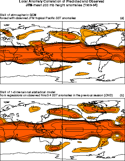
The rough agreement between the two panels in Fig. 2.4 may be interpreted as reflecting either true seasonal predictability limits or the need for further GCM improvement. There is room for both interpretations, although we are more inclined toward the former. GCM error is probably not the main culprit here: several other GCMs analyzed by us yield skill patterns very similar to that in the upper panel. Also, when the NCEP GCM is asked to predict its own behavior, such as when using an 8-member ensemble-mean to predict the 9th member's seasonal anomalies, its skill is again similar to that in the upper panel. One can thus make a case that the modest extratropical values in Fig. 2.4 are mainly a reflection of the limited intrinsic predictability of extratropical seasonal averages associated with tropical SST forcing. As mentioned earlier, this in turn is mainly due to a modest signal-to-noise ratio.
CDC scientists have attempted to clarify the relationship between the
expected anomaly correlation skill  of ensemble-mean forecasts and the
signal-to-noise ratio s, defined as the ratio of the
ensemble-mean anomaly to the ensemble spread. Figure
2.5 summarizes this general relationship, which is useful in
interpreting many GCM results. The
  and
and  curves show the expected skill of
infinite-member and single-member ensemble-mean forecasts with a
perfect model. The third (blue) curve depicts the expected skill of
infinite-member ensemble-mean forecasts with an imperfect model, whose
systematic error se (i.e., its error in determining
the true s) is of the same magnitude as s. Note that
these curves are applicable to any forecast variable, in any
forecasting situation, and to any forecasting method, including the
regression method used in Fig. 2.4b.
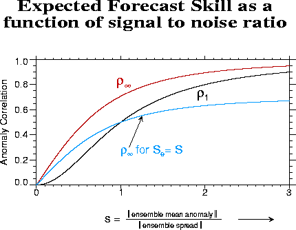
The  curve
represents a hard predictability limit with a perfect model, and shows
that to produce 'useful' forecasts with anomaly correlations greater
than 0.6, s needs to be greater than 0.75. To produce
'excellent' forecasts with anomaly correlations greater than 0.9,
s needs to be greater than 2. Given the evidence from several
studies that s for ENSO-related 200 mb seasonal height
anomalies is approximately between 0.5 and 1 in the extratropical
Pacific-American sectors of both hemispheres, and greater than 2 in
the tropics, the results in Fig. 2.4 are not
surprising. Figure 2.5 is also useful for
assessing to what extent the modest skill in Fig. 2.4a might be due to model error or using only
9-member ensembles. The difference between
  and
and  shows the potential gain in
skill by using infinite-member ensembles instead of a single
member. The maximum gain is 0.25, for s ~ 0.6. However, most of
this gain is attainable with about 25 members, and even a
  curve (not shown) is close to
the curve. The loss of skill due to model error (blue curve) is
probably of greater concern in Fig. 2.4a than
not having enough members. However, model error could equally be
affecting skill in Fig. 2.4b.
2.2.2 New research challenges
Figures 2.4 and 2.5 together suggest that the modest skill, on average, of deterministic extratropical seasonal forecasts is largely consistent with the predictability limits imposed by the modest local values of s associated with the tropically forced signal. Given also the evidence in Fig. 2.4b that similar skill can also be achieved with simple linear regression models, the question naturally arises as to what further useful predictive information can be extracted by running GCM ensembles.
CDC scientists have spent considerable time pondering this issue, and have come up with several encouraging possibilities. In one way or another, they all involve focusing on the distributional aspects of the ENSO response rather than on the ensemble-mean. For example, as Fig. 2.6a shows, a modest shift in the mean of 0.5 (in units of standard deviation), while not large enough to affect appreciably the expected seasonal mean of an extratropical variable, can still greatly affect the probability of its extreme values. The risk of obtaining an extreme positive value of greater than +1 increases from 16% to 31%, and the risk of obtaining an extreme negative value decreases from 16% to 7%. Thus without ENSO the risks of extreme positive and negative anomalies are the same, but with ENSO, even for a modest s of 0.5, the risk of an extreme positive anomaly becomes 4.4 (=31/7) times the risk of an extreme negative anomaly. Figure 2.6b shows how this risk ratio can be equally strongly affected by modest changes of noise. In this example, a 20% reduction of standard deviation combined with a mean shift of 0.5 changes the risk ratio from 1 (=16/16) to 9 (=27/3).
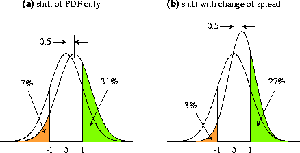
When even minor PDF shifts and changes of variance imply large changes in the risks of extremes values, determining them accurately becomes important. It is easy to see how a good GCM might have an advantage over the regression model of Fig. 2.4b in this regard, whose parameters cannot be estimated accurately enough from the limited observational record to have confidence in its predictions of extreme values. Further, one can run as many GCM ensemble members as necessary in individual forecast cases to predict the changes of extreme risks within specified confidence intervals. The regression-model also assumes, in effect, that ENSO-induced mean PDF shifts are strictly linear with respect to the SST forcing and that there are no changes of noise, or variability. CDC scientists have spent considerable effort on ascertaining the extent to which such assumptions are valid, since they have a large bearing on the problem at hand.
2.2.3 Understanding the sensitivity of the atmospheric response to details of the anomalous SST forcing
The regression-model used in Fig. 2.4b always predicts the same signal pattern of the global atmospheric response; only its amplitude varies from forecast case to case in direct proportion to the strength of the Niño 3.4 SST anomaly. As we have seen, this doesn't seem to affect its deterministic forecast skill overmuch, but the question is whether it limits predictions of the risk of extreme anomalies. To what extent does the remote SST-forced signal vary from case to case? To what extent are its variations determined by the nonlinearity of the response to the amplitude and sign of the SST forcing in Niño 3.4, and to what extent by the details of the SST anomaly pattern in the wider tropical Indo-Pacific domain? We have conducted several studies to answer these questions.
Figure 2.7 gives a sense of the signal variation from case to case. Sampling uncertainty is an issue in this problem, given that the number of samples required to establish that s is statistically different from zero is inversely proportional to the square of s. At the 5% level, the number of samples should be greater than 8/s2. To establish the significance of s = 0.5 thus requires 32 samples; to establish the significance of changes of s from case to case, say of order 0.25, would require many more, 128. With this in mind, we ran a very large 180-member seasonal ensemble with the NCEP atmospheric GCM with prescribed observed global SST forcing corresponding to the El Niño of 1987, and another 180-member ensemble for the La Niña of 1989. The right-hand panels of Fig. 2.7 show the ensemble-mean 500-mb height anomalies obtained in these integrations (defined with respect to the ensemble-mean obtained in another set of 180 integrations with climatological-mean SST forcing). To our knowledge this is the most statistically confident determination of the global SST-forced signal ever made for two different observed SST forcing patterns. Note that the sign of the response has been reversed in the lower panel for easier comparison with the upper panel. For comparison we also show in the left panels, in an identical format, observational 500-mb composite anomaly patterns for 10 El Niño and 10 La Niña events based on the Niño 3.4 index, and defined with respect to 10 "neutral" events. Note that the amplitudes of these composite patterns have been scaled by 0.73 and 1.36, in proportion to the observed Niño 3.4 SST anomaly magnitudes during the moderate 1987 El Niño and the strong 1989 La Niña events, respectively. Thus these left panels may be interpreted as the SST-forced 500-mb height signals during 1987 and 1989 as predicted by an empirical method. This method is superior, in principle, to that used in Fig. 2.4b in that it predicts different response patterns in El Niño and La Niña cases, as shown here.
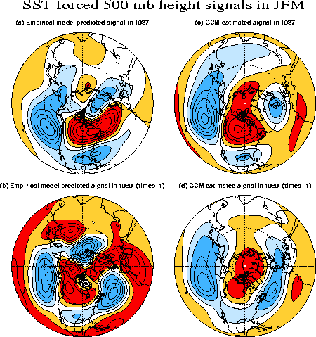
Although the GCM's signal patterns for these individual El Niño and La Niña winters are generally similar to one another, there are some notable differences. The El Niño response is stronger in the PNA sector, despite the weaker SST forcing. This is also true in the empirical forecast. There is little else to compare between the GCM and empirical forecasts because of sampling uncertainty in the empirical forecasts, i.e., the fact that the left panels are derived from only 10 cases each in the historical record. In areas such as the North Atlantic where the left panels predict a strong asymmetric signal of the same sign in 1987 and 1989, the significance of that asymmetry is therefore questionable. The differences between the GCM's predicted signal patterns for 1987 and 1989 are much more reliable in this regard, and though more modest, are large enough that they would have had important implications for predicting the risks of extreme anomalies during these winters.
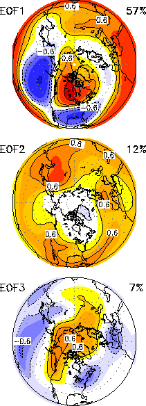
There is thus evidence of significant signal variation from case to case. To put these results on a stronger footing, one might ideally wish to generate similar 180-member ensembles for each one of the past 50 or so winters. This has not yet been done. However, results from a 46-member multi-model ensemble of four different atmospheric GCMs (NCAR CCM3, NCEP, GFDL, and ECHAM) offer additional evidence of the existence of different response patterns. Between 10 and 12 member ensembles were generated for each model forced with identical evolving observed global SSTs over the past 50 years. For each one of the 50 winters, the SST-forced signal at 500 mb was defined as a weighted average of the ensemble-mean responses of the 4 GCMs. Finally, an EOF analysis of these 50 signal patterns was performed. Figure 2.8 shows the first three EOFs, together with their fractions of the total signal variance explained. The leading EOF alone accounts for 57% of the global signal variance, and as much as 80% over the PNA region. Most elements of this pattern are evident in all the four panels of Fig. 2.7. The dominance of this signal pattern, its strong similarity to the classic observed ENSO teleconnection pattern, and also to the unchanging forecast pattern of the regression model used in Fig. 2.4b, explains why the upper and lower panels of Fig. 2.4 are so similar. Still, there is evidence in Fig. 2.8 of apparently minor but potentially important deviations from this dominant signal pattern from winter to winter. The second EOF is largely zonally symmetric, with out-of-phase anomalies in polar and subtropical latitudes. Locally, it explains a substantial fraction of the signal variability in the subtropics, and its associated Principal Component (PC) time series describes a tropospheric warming trend of lower latitudes over 1950-1999 associated with a long-term tropical SST warming trend. The third EOF resembles a tropically forced wavetrain with centers spatially shifted relative to those of the leading EOF. Its PC time series regressed on the simulated tropical precipitation fields yields a regression map with appreciable magnitudes in the western and central equatorial Pacific. This third EOF may thus reflect a genuine sensitivity of the SST-forced extratropical signal to variations of the anomalous tropical SST pattern from winter to winter.
It should be stressed that the GCM results in Figs. 2.7 and 2.8 are all for global SST forcing. To what extent can the signal variation evident in these figures be attributed strictly to the tropical Pacific SST forcing, in particular to asymmetric responses to El Niño and La Niña forcing? There is a strong suggestion of a weaker response to La Niña forcing in the lower panels of Fig. 2.7. Such a weaker response (not shown) is also clearly evident in the composite El Niño and La Niña signals in the 4 different ensemble GCM simulations for 1950-1995 described above. Are there also significant differences in the patterns of the response? To what extent do they contribute to the third EOF in Fig. 2.8? Several CDC studies have attempted to address such questions cleanly, by examining the atmospheric response to the first EOF pattern of tropical Pacific SST (very similar to the Pacific portion of the lower panel of Fig. 2.1) with positive ("El Niño") and negative ("La Niña") signs. A weaker response to the negative EOF forcing has indeed been confirmed, but is appreciable only for large amplitude forcing.
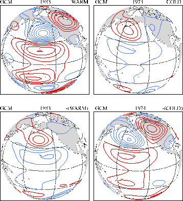
Figure 2.9 shows results from a GCM experiment designed specifically to address this issue. A 9-member NCEP GCM ensemble was generated for 1963-1989 by forcing throughout the 27 years with the first SST EOF pattern, varying in magnitude and sign as its associated PC time series. The upper panels of Fig. 2.9 show the ensemble-mean responses during the strongest warm and cold winters of 1983 and 1974, respectively, in this period. The response is clearly weaker for the 1974 event. This is suggestive but not conclusive, since the magnitude of the SST forcing was also weaker in 1974. To settle this, the entire experiment was repeated with the sign of the PC time series reversed. The ensemble-mean responses for the sign-reversed 1983 and 1974 winters are shown in the lower panels. The 1974 response is now stronger than the 1983 response, despite the weaker magnitude forcing. We had noted this effect earlier in Fig. 2.7, but the result here is cleaner. It confirms that the remote atmospheric response to the tropical Pacific SST forcing is appreciably stronger for strong warm than for the strong cold SST forcing. A top-to-bottom comparison in Fig. 2.9 compares the responses to the same SST forcing but of opposite sign, and further confirms this result.
2.2.4 ENSO-induced changes of variability
To what extent does ENSO affect the atmospheric noise (i.e., the
variability) as hypothesized in Fig. 2.6b? We
have addressed this issue in several recent publications. In one
study, we examined the standard deviation of seasonal-mean 500 mb
heights in our 180-member GCM ensembles for the winters of 1987 and
1989, and found a modest overall increase in the warm (1987) and a
decrease in the cold (1989) ensemble compared to that in the neutral
180-member ensemble. This was speculated to be forced partly by the
increased variability of seasonal precipitation in the warm (and
decreased variability in the cold) ensemble in the Niño-4 area of the
central equatorial Pacific, which has been shown to be sensitive
region for forcing a large global circulation response. Another study
searched for ENSO-induced changes of seasonal noise in the smaller
AMIP-style GCM ensembles used in Fig. 2.8, but
found little impact in the PNA region. While these findings seem to
conflict, a closer look at the published figures shows that the
results are not inconsistent in the PNA region. To the extent that the
altered extratropical noise is due to the tropical precipitation
noise, the effect is also probably both GCM-dependent and ENSO
event-dependent. It should be mentioned that sampling uncertainty is
of even greater concern here than in Figs. 2.7
and 2.8. The number of samples required to
establish the significance at the 5% level of a fractional change  of an ensemble's standard
deviation is close to 3/
 . To establish the significance of the
  of 0.2 (corresponding to a 20%
change of standard deviation) in Fig. 2.6b would
thus require 75 samples from both the neutral and altered
distributions. Any change of smaller than 17.5% would require more
than 100 samples.
The effect of ENSO on subseasonal extratropical variability is equally important, and somewhat easier to establish. These effects can be distinct from the effects on seasonal mean quantities, and can have important practical implications. For instance, one may imagine a situation in which El Niño alters the occurrence of both cold waves and warm spells in a winter. The effect is a meaningful change in the risk of extreme weather, even though little seasonal mean signal might be evident. The few published studies on this topic, constrained either by sampling requirements or data availability, have formed composites over several ENSO events to diagnose the effect in limited regions. In an ambitious recent study, we have estimated the effect globally from our large AGCM ensembles for 1987 and 1989, and compared them with observational composites based on 11 El Niño and 11 La Niña events in the recent record. As in Fig. 2.7, the purpose of this comparison was to gauge to robustness of the changes of variability, their predictability, and their variation from event to event.
The most important result from this analysis, depicted in Fig. 2.10, is that the patterns of the SST-forced
anomalous height variability are markedly different for the synoptic
(2 to 7 days), intraseasonal (8 to 45 days), and monthly (30 -day
average) time scales. In contrast, the patterns of the anomalous
tropical rainfall variability (not shown) are nearly identical across
these time scales. Figure 2.10 shows contours
of  , defined as
the signed square root of the anomalous variance difference of 500 mb
heights on these time scales (where by "signed" we mean that if the
anomaly is negative, we depict its square root with a minus sign). The
results for La Niña (not shown) are similar and generally of opposite
sign. The comparison between the GCM and observational panels in Fig. 2.10 is not clean. Nevertheless, their gross
similarity is reassuring, both for the robustness of the changes of
variability and this GCM's ability to simulate them. To that extent,
their dissimilarity can be attributed to the comparison not being
clean (i.e., event-to-event differences) and sampling error,
especially in the observations (which is why the observational
anomalous monthly variability map has been omitted).
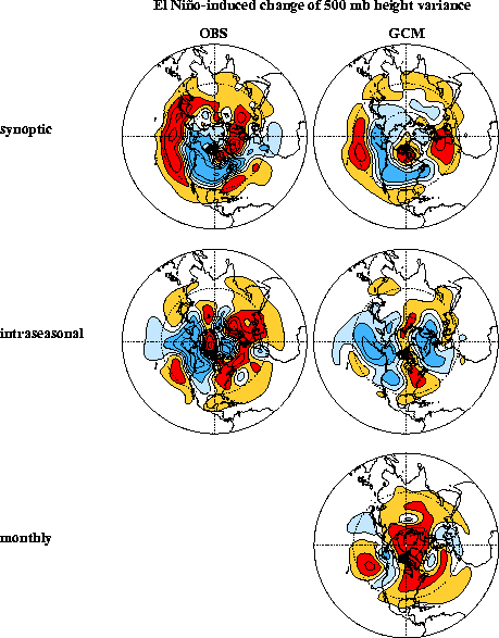
The main ENSO effect on the synoptic scale is a southward shift of the storm track over the Pacific ocean and North America. On the intraseasonal scale, it is a decrease of height variance over the north Pacific, consistent with a tendency of reduced blocking activity during El Niño. On monthly (and seasonal) scales there is a suggestion of an overall increase of variance. Referring back to Fig. 2.6b, it is evident that these differing ENSO impacts on extratropical noise on different time scales have very different implications for the risks of extreme anomalies on these scales. We believe that three quite distinct dynamical mechanisms are responsible for these sharp differences, and are currently investigating them in a hierarchy of dynamical models.