2.4 Understanding and predicting SST variations outside the tropical Pacific
2.4.1 The atmospheric bridge
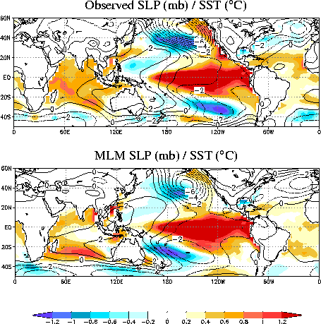
One example of global climate interaction is the "atmospheric bridge", where atmospheric teleconnections associated with ENSO drive anomalous ocean conditions outside of the equatorial Pacific through changes in the heat, momentum, and fresh water fluxes across the air-sea interface. The resulting SST anomalies can also feed back on the initial atmospheric response to ENSO. As part of the GFDL-Universities Consortium project, we developed a coupled AGCM-mixed layer ocean model and used it to conduct experiments to study the atmospheric bridge and other air-sea interaction processes. In the "MLM" experiment, observed SSTs were prescribed as boundary conditions in the tropical Pacific (15N-15S, 172E-South American Coast), and the remainder of the global oceans were simulated using the variable-depth mixed-layer model. As Fig. 2.12 shows, the simulated SLP and SST anomalies associated with ENSO are fairly realistic, with stronger cyclonic circulation and cold water over the central North and South Pacific and warm water along the west coast of the Americas. ENSO-induced changes in the Walker circulation also lead to warm SSTs in the north tropical Atlantic and Indian Oceans.
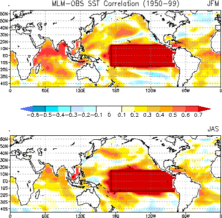
How useful is this effect in actually predicting the interannual variations of SSTs outside the tropical Pacific basin? Figure 2.13 provides one measure of the forecast skill. It shows the correlation of the observed seasonal-mean SST anomalies, over the 50-year 1950-1999 period, with those predicted by the MLM model. The predicted field for each season represents a 16-member ensemble-mean. Results are shown separately for the 50 winter (JFM) and 50 summer (JAS) forecast cases over which the correlations were calculated. The correlations are generally higher than 0.4 in the central north and south Pacific oceans, and also in the tropical Indian and tropical Atlantic oceans. This is encouraging, and also sheds some light on why the LIM SST forecast models described in section 2.1, that are based solely on SST correlations between different tropical locations, perform as well as they do: the "bridge" effect is implicitly included in them. It is also interesting to compare Fig. 2.13 with Fig. 2.12 in areas such as the north Atlantic, where Fig. 2.12 suggests a bridge effect but Fig. 2.13 shows it to be unimportant.
2.4.2 The re-emergence of long-lived subsurface temperature anomalies
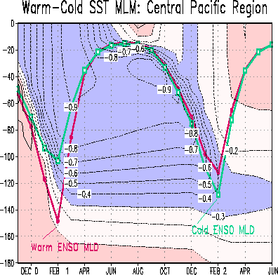
The atmospheric changes associated with ENSO influence upper-ocean processes that affect the subsurface temperature structure and mixed-layer depth (MLD) long after the ENSO signal decays. Thermal anomalies that form in the surface waters of the extratropics during winter partially reemerge in the following winter, after being sequestered beneath the mixed layer in the intervening summer. SST anomalies generated via the atmospheric bridge recur in the following winter in central North Pacific via this reemergence mechanism (Fig. 2.14). The MLD is substantially deeper in the central North Pacific during El Niño than La Niña winters, but the reverse is true in the subsequent winter. During El Niño winters, enhanced buoyancy forcing (surface cooling) and mechanical mixing creates a colder and deeper mixed layer. After the MLD shoals in late spring, the cold water stored beneath the surface layer as part of the reemergence process increases the vertical stability of the water column, reducing the penetration of the mixed layer in the following fall and winter.
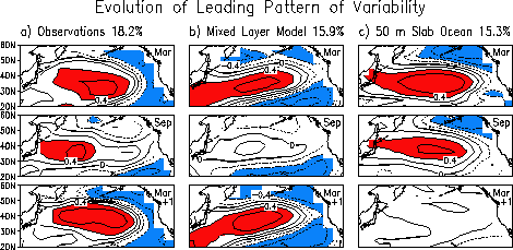
The reemergence process is not confined to the central North Pacific, nor does it occur solely in conjunction with the atmospheric bridge. Figure 2.15 shows the evolution of the leading pattern of North Pacific SST variability in observations and in two distinct AGCM - ocean model experiments. In the first experiment, the mixed layer ocean model is active over the entire globe, including the tropical Pacific, and thus does not include ENSO. In the second experiment, observed SSTs are specified in the tropical Pacific, but the remainder of the world oceans are simulated by a slab model without mixed-layer physics. The observational column in Fig. 2.15 shows that the dominant large-scale SST anomaly pattern that forms in the eastern two-thirds of the North Pacific during winter recurs in the following winter without persisting through the intervening summer. Experiment 1 (middle column) reproduces this behavior, but Experiment 2 (right column) does not. These results suggest 1) that the winter-to-winter SST correlations are due to the reemergence mechanism and not due to similar atmospheric forcing of the ocean in consecutive winters, and 2) that the SST anomalies in the tropical Pacific associated with El Niño are not essential for reemergence to occur.