3.5 Experimental week 2 forecasts of extreme events using the operational NCEP ensemble

The existence of a significant spread-skill relationship (at relatively short forecast ranges) means that changes of both the mean and width of the forecast probability distribution from their climatological values can be used to estimate the probability that the verification will lie in the tails of the climatological probability distribution (see Fig. 2.6). The statistical models discussed earlier assume that the spread is constant, and that only shifts of the mean are important in altering the probability that the verification will be an "extreme event".

Unfortunately, this advantage of ensemble forecasts, which is modest but significant in Week 1, is lost by the middle of Week 2. The main reason is that by Week 2 the forecast ensemble spread nearly saturates to its climatological mean value, so that there are no significant spread variations from case to case. In other words, most of the predictable variation of forecast skill in Week 2 is associated with predictable variations of the signal, not of noise. For several years CDC has exploited this fact in producing an experimental real-time Week 2 forecast product based on the NCEP ensemble (http://psl.noaa.gov/~jsw/week2/). Tercile probability forecasts of 500 mb height, 850 mb temperature, 250 mb zonal wind, sea-level pressure and precipitation are provided. Only the signal, not noise, is used to construct these probability forecasts. The procedure involves converting maps of the predicted standardized anomalies into maps of extreme quantile (in this case, tercile) probabilities. This calibration is done empirically, using the available historical record of ensemble forecasts and verifying analyses. The procedure is as follows: 1) for a positive standardized forecast anomaly , all instances in which a forecast exceeded this value in the data record are found, and the probability that the verifying analysis fell in the upper tercile of the climatological distribution is computed, 2) the standardized anomaly contour is relabeled as a probability of above-normal equal to . If is negative, the probability that the verifying analysis fell into the lower tercile is computed, and the contour is relabeled "probability of below-normal". If the model has systematic errors, these probabilities need not be symmetric, i.e. the probability of below-normal for a negative need not be the same as the probability of above-normal for a positive . Our calibration thus provides one simple way of accounting for model error in probabilistic predictions.

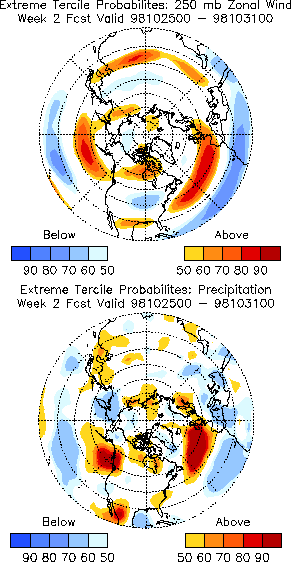
Figure 3.11 shows an example of such a probability forecast. Note that the interpretation of this map is slightly different from that for a conventional probability forecast. If all the points on the map inside the yellow contour (as opposed to those inside the yellow band) are counted over a large sample of forecasts, 50-60% of these points will verify in the upper tercile of the climatological distribution. Similarly, for points falling in the darkest red regions on the map, over 90% will verify in the upper tercile. The conventional interpretation would be that points in the yellow band would have a 50-60% chance of verifying in the upper tercile. Such a calibration would require a lot more forecasts to compute reliably, since there are far fewer points inside the yellow band than there are inside the yellow contour.

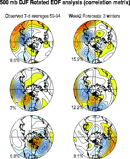
Since we assume that the signal, not the noise, contains all of the useful predictive information, the useful subspace of the ensemble can be isolated through an EOF analysis of the correlation matrix of the ensemble-mean predictions. (The idea here is similar to that in Fig 2.8). The right panels of Fig. 3.12 show the three leading EOFs thus obtained. For comparison, the three leading EOFs of the correlation matrix of observed 7-day averages is also shown, in the left panels. There are two notable aspects to Fig. 3.12: 1) the signal and observed EOF patterns are similar, and 2) the three leading EOFs explain considerably more variance of the ensemble-mean forecasts than they do of the observed variability (36% vs. 22%). To understand this better, note that the total forecast covariance can be decomposed into a part due to the predictable signal (C_signal) and a part due to unpredictable noise (C_noise). If the forecast model is unbiased and the noise is uncorrelated with the signal, the observed variance (C_obs) is approximately the sum of the two. This relationship is exact for the LIM discussed in section 3.1. The fact that the signal variation occurs in a lower dimensional subspace than the observational 7-day averages then simply means that the variance contained in the noise is non-trivial. The similarity of the observed and signal EOF patterns has a subtler interpretation: it implies that the noise component of the covariance is nearly white, and that the ensemble-mean does indeed capture most of the extractable signal with coherent spatial structure.

The product shown in Fig. 3.11 has been quite popular with operational forecasters. A similar method has been adopted in operations by NCEP/CPC. A detailed analysis of the performance of this scheme, and its implications for Week 2 predictability, is underway.

Back | Forward